Recently I wanted to learn more about ocean emulators, so I decided to build my own. Given my lack of experience working with emulators and time for this kind of pursuit I decided to see how far I could push using AI to generate the code and develop a self-improving process for improving the output. Within a few weeks of starting this side project I had generated this emulator of a two-layer shallow water double gyre model where the original model is on the left and the emulator output (called Rollout) is on the right. To get to this point I ran through hundreds of different model configurations and generated an app to track the model outputs. In this post I share what I learned in this process.
So what was the goal?
My goal was to build a process that could continually improve some kind of benchmark model. In my case I decided that the model would be an ocean emulator.
Why an emulator project?
Firstly, with an emulator project the source data is the output from another ocean model - in this case the Aronnax shallow water model made by Ed Doddridge. With ocean model output there is no ambiguity about the trustworthiness of the data and so no judgement calls for the model to make on which potential outliers to keep or remove, as these judgement calls are a real weakness of contemporary models.
Secondly, with an emulator project we can make a lot of progress with a single evaluation metric - the root-mean-square (RMS) distance between the original model and the emulator output. At the end of every iteration this metric is passed to the LLM and if the number goes down then we’re probably making progress. Eventually, further metrics will be required to judge progress such as spectral properties but at the outset the RMS distance is a good indicator.
Thirdly, emulator projects build upon a large public literature on developing deep learning models across much wider domains than geophysical fluid mechanics such as computer vision. LLMs have an excellent knowledge of what works from this literature and can make confident hypotheses on how to make progress from the current point.
Problem domain
The ocean model I looked to emulate was a shallow water model in a double-gyre set-up. I did the initial experiments with a one-layer model and then moved to a more dynamic two-layer once the initial problem was solved.
I chose this relatively simple domain as I was primarily focused on how to build an autodiscovery pipeline rather than a frontier ocean emulator. While this domain is relatively simple compared to emulating a global ocean model it is still not a trivial problem - numerous automated pipelines that I started failed to develop into a useful emulator.
A classic double-gyre model has a fixed wind field. I wanted to ensure the agent had to learn how to handle some kind of time-varying surface boundary condition so I created a surface wind field that shifts north and south periodically over the course of each year. The ocean model run was 5000 days. This was long enough to train an emulator on but short enough to maintain a fast iteration pace in the emulator development pipeline.
Auto-discovery pipeline
Agent harness
In this project the underlying LLM I used throughout was the Codex LLM from OpenAI. However, for the coding harness I used the open source Pi.dev framework. The Pi.dev framework provides more control over what is sent to the LLM compared to a proprietary harness as it implements a minimal system prompt.
Using Pi.dev was particuraly useful in terms of making the model more willing to do many repeated iterations. In my early attempts it was challenging to get the model to kick off a new iteration at the end of experiment.
With some back and forth interactions with the model I learned that this reticence was because the LLM has built-in instructions to be conservative in terms of resources (e.g. tokens or API calls) used. When I added targetted instructions for it to instead be aggressive in terms of resource use I found the model was then able to continue generating new experiments over the course of hours at a time.
Project set-up
The project used an approach known as autoresearch. In this paradigm:
- we define an overall metric that the model is evaluated on
- we keep a markdown file where the agent keeps tracks of the results to date
- each step of the process is an experiment associated with a given hypothesis that is generated by the agent
- every experiment is associated with a git branch
- at the end of every experiment the agent writes the key results to a central markdown file
- if a branch provides a new benchmark result then its results are merged back into the main branch to replace the existing benchmark
A key aim of this process is to ensure that any results arrived at along the way are fully reproducible. This autoresearch approach is in contrast to a simpler alternative for persistent tasks where we use built-in functionality such as /loop in claude code. In that case the agent manages the experiments (rather than git and the markdown) and it is easy to end up with earlier results that can no longer be reproduced later.
Hypothesis generation
In my initial efforts I let the agent generate each new hypothesis. Giving the agent full control over hypothesis generation provided poor results as the agent had a strong bias towards making very small configuration adjustments (e.g. changing the size of a layer or a learning rate) which resulted in approaches that quickly reached dead ends.
Successful results require a balance between making bigger jumps in architecture and then exploring within each of these architectures to see if promising results can be developed. This process is familar to any scientist - while we want to try different approaches we also know that results are generally not instantaneous and that persistence is required with any hypothesis to maximise its performance.
I found that although agents have a strong bias towards low-risk low-reward configuration adjustments they could also produce a list of high-risk high-reward alternatives. I then started a session by asking the agent to produce such a list of 40 or 50 hypotheses graded by risk/reward level. When the agent was set to the task of developing a better model it was instructed to evaluate recent results to see if the current hypothesis is worth peristing with. If a plateau had been reached it was instructed then to review the list and choose an alternative hypothesis.
Results
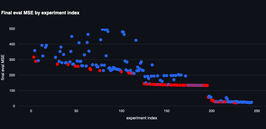
I triggered the autoresearch approach for the single-layer double gyre simulation. With the approach set out above the following set of results in terms of the evaluation metric was arrived at. Experiments with a metric greater than 500 are excluded.
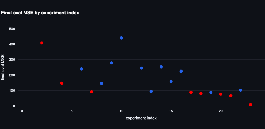
I then moved on to the double-gyre simulation where the extra layer makes the simulation more turbulent. The results are shown here with the first two simulations with an evaluation metric not shown as they are above the cutoff of 500.